Linear Systems of Equations

Linear Systems of Equations
A system of equations (you know this), where every term is a scalar multiple of a variable. Then, each equation models a linear combination of the variables.

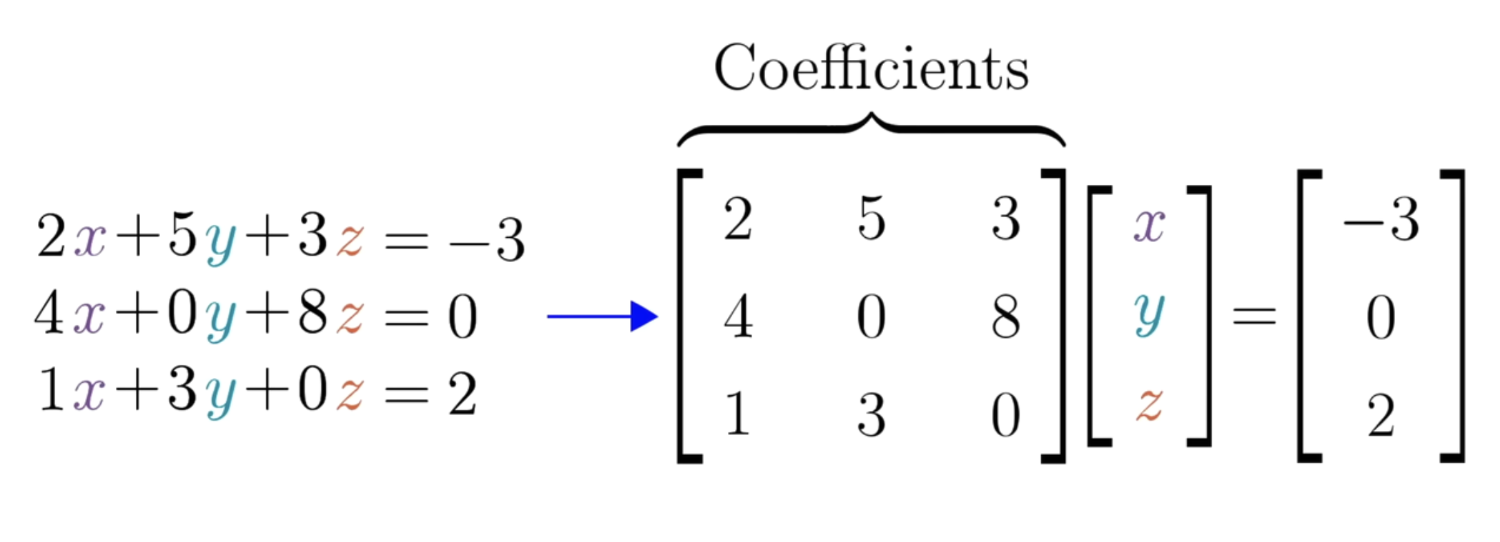
Credit to 3Blue1Brown.

This can be written as $A\cdot \vec{x}=\vec{v}$. So the solution to a system of linear equations is just a vector that, when transformed by $A$, gives $\vec{v}$! How do we solve a system of linear equations (SLE)? We can use Gaussian elimination: we write the SLE as an augmented matrix, row reduce it, and then solve the resulting system of equations.
First, let's note that a system of linear equations will have either zero, one, or infinitely many solutions:

Theorem: Suppose $x_1$ and $x_2$ are solutions to the matrix equation $A\vec{x}=\vec{b}$. If $\alpha$ and $\beta$ are any real numbers such that $\alpha + \beta=1$, then $\alpha x_1 + \beta x_2$ is also a solution to the equation.

Here are some important terms we need before we can solve SLEs:

Consistent
A linear system of equations is consistent if it has at least one solution. Otherwise, it is inconsistent.

Homogenous
A system of linear equations corresponding the matrix equation $A\vec{x}=\vec{b}$ is homogenous if $\vec{b}=\vec{\textbf{0}}$. Otherwise, it is inhomegenous. Every homogenous system is consistent ($\vec{x}=\vec{\textbf{0}}$, which is called the trivial solution).

Row-Reduced Form
A matrix is in row-reduced form if it satisfies the following four conditions:

1. All zero rows (if any) appear below all nonzero rows.
2. The first nonzero element in any nonzero row is $1$.
3. All elements below and in the same column as the first nonzero element in any nonzero row are $0$.
4. The first nonzero element of any nonzero row appears in a column further (farther??) to the right than the first nonzero element in any preceding row.

Ex. $A=\begin{bmatrix}1 & 7 & -1 \\ 0 & 1 & 6 \\ 0 & 0 & 0\end{bmatrix}$ is in row-reduced form.

Pivot
If a matrix is in row-echelon form, then the first nonzero element of each row is called a pivot, and a column in which a pivot appears is called a pivot column. In a system of linear equations, the pivot columns represent basic variables. Non-basic variables (ones that are not in a pivot column) are called free variables. Free variables can take on any value (we are "free" to choose any value)

Now we're ready to solve SLEs!

The first thing we need to do is form an augmented matrix. This is a matrix that has the coefficients of the variables on the left and the constants on the right. For example, the augmented matrix of the system $$\begin{align}x_1+2x_2+3x_3&=4\\2x_1+5x_2+2x_3&=3\\3x_1+7x_2+8x_3&=1\end{align}$$ is $$\begin{bmatrix}1 & 2 & 3 & 4\\2 & 5 & 2 & 3\\3 & 7 & 8 & 1\end{bmatrix}.$$

Once we've constructed this augmented matrix, we can use Gaussian elimination to row reduce it. This involves using elementary row operations to transform the augmented matrix into row-reduced form.

Guassian Elimination
First, note that the following three operations do not change the set of solutions:

1. $R_1$ — Changing the order of equations.
2. $R_2$ — Multiplying an equation by a nonzero scalar.
3. $R_3$ — Adding to one a equation a scalar times another equation.

These are called elementary row operations. We'll talk more about them in a later section. The augmented matrix of the system $A\vec{x}=\vec{b}$ is $\left [A\;\textbf{|}\;\vec{b} \right]$. Guassian elimination has 4 steps:

1. Write the system of equations as an augmented matrix.
2. Use elementary row operations to transform the augmented matrix into row-reduced form.
3. Write the equations corresponding to the reduced augmented matrix.
4. Solve the new set of equations with back-substitution.

Here are some general guidelines for working with elementary row operations:

• Completely transform one column into the required form before starting on another.
• Work the columns in order from left to right.
• Never use an operation that changes a $0$ in a previous column.

If the number $n$ of variables is greater than the number $r$ of variables, then the $r$ equations determine the values of $r$ variables, and the remaining $n-r$ variables have no restrictions. Thus, there are infinitely many solutions. Once we've row-reduced the augmented matrix, we can write the system of equations corresponding to the reduced augmented matrix. We can then solve this system of equations using back-substitution. For example: $$\begin{align}x_1+2x_2+3x_3&=4\\2x_1+2x_2+2x_3&=2\\3x_1+6x_2+9x_3&=12\end{align}$$ The augmented matrix is $$\begin{bmatrix}1 & 2 & 3 & 4\\2 & 2 & 2 & 2\\3 & 6 & 9 & 12\end{bmatrix}.$$ The row-reduced form of the augmented matrix is $$\begin{bmatrix}1 & 2 & 3 & 4\\0 & 1 & 2 & 3\\0 & 0 & 0 & 0\end{bmatrix}.$$ The corresponding system of equations is $$\begin{align}x_1+2x_2+3x_3&=4\\x_2+2x_3&=3\\0&=0\end{align}$$ The last equation is a trivial equation and doesn't provide any new information. So, we can ignore it. We can then solve the remaining two equations using back-substitution.

Elementary Matrices
An elementary matrix $E$ is a square matrix such that multiplying it by $A$ on the left is the same as applying an elementary row operation to $A$. Elementary matrices are easily constructed by applying the corresponding elementary row operation to the identity matrix of the same order. So, the elementary matrix that corresponds to multiplying the first row of an $n\times n$ matrix by $k$ is $$\begin{bmatrix}k & 0 & 0 & \dots & 0\\0 & 1 & 0 & \dots & 0\\0 & 0 & 1 & \dots & 0\\\vdots & \vdots & \vdots & \ddots & \vdots\\0 & 0 & 0 & \dots & 1\end{bmatrix}.$$

LU Decomposition
If a nonsingular (invertible) matrix $A$ can be written as the product of a lower triangular matrix on the left and an upper triangular matrix on the right, $A$ is said to have an LU decomposition. Let $R_3(i,j,k)$ denote the elementary row operation that adds $k$ times the $j$th row to $i$ where $k\neq 0$ and $i\neq j$. We know that the matrix $R_3(i,j,k)$ has all diagonal elements equal to $1$, element at $(i,j)$ equal to $k$, and $0$ everywhere else. So, if $i>j$, $R_3(i,j,k)$ is a lower triangular matrix. All diagonal elements of a square $n\times n$ nonsingular lower triangular matrix $L$ must be nonzero. A nonsingular $n\times n$ matrix $A$ has an LU decomposition if and only if $A$ can be transformed into an upper triangular matrix with $R_3(i,j,k)$ where $i>j$. A square matrix $A$ has an LU decomposition if $A$ can be transformed to an upper triangular matrix using only the third elementary row operation. If $A$ has an LU decomposition, we can solve the equation $A\vec{x}=\vec{b}$ by solving $L\vec{y}=\vec{b}$ and the equation $U\vec{x}=\vec{y}$. Then, we would have $LU\vec{x}=\vec{b}$, $L\vec{y}=\vec{b}$.